Multiplicative Model: Trend and Seasonality with Excel

Trend or seasonality? If the data shows that sales of eggnog dropped in January, we would suspect the data reflects seasonal influences rather than a downward trend. If the sales of sherbet increased in July, we would likely have the same suspicion. However, depends on product category, trend and seasonality aren’t always this simple to decipher.

To accurately forecast sales when the data has seasonality and trends, we’ll need to identify and separate them from the data series. Sometimes it is as simple as using moving averages to smooth data and eliminate seasonality (e.g. excel scatter plot with trend line. When monthly seasonal influence is suspected, use a 12-month moving average, when analyzing trend in quarterly data, use a four-quarter moving average). Yet, sometimes it is more complicated than that.

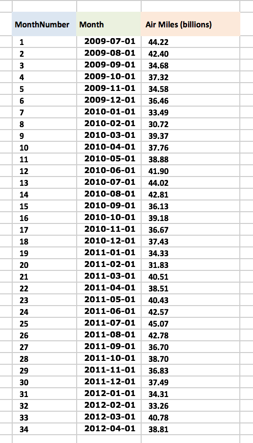
Today, I would like to practice building a multiplicative model with this classic air miles data with excel solver. First, we will have to set up trial values for base, trend and seasonal indices.

The base is the best estimate of the level of monthly airline miles without the influence of seasonality. The trend represents the percentage monthly increase in the level of airline miles. Lastly, the seasonal index represents the percentage by which airline travels for the month is above or below an average month.

We will also need to add an extra column for month, this is for the convenience of setting up VLOOKUP. After that, we can start plug in the forecasting equation. Predicted Period t sales= Base*(Trend^t)* (Seasonal Index for month t)

Compute the monthly forecast’s error (forecast- air miles), squared error and the Sum of Squared Errors.

Now we can set up the Solver. Our objective is to minimize the Sum of Squared Errors $J$7, by changing variable cells of base, trend, and the twelve seasonal indices, $B$2:$B$3, $B$5:$B$16 in this case. Our model subjects to the constraints of $B$18=1, $B$5:$B$16<=3, base<=100, and trend<=2. The constraint $B$18=1 is to make sure seasonal indices average to 1. Run GRG Nonlinear solver.

Now we have our results. The estimated base level of airline miles (red) is around 37.4 billion. We can estimate the trend by computing trend^12-1 and it will give us an increase of 0.15% per month (1.8% per year). As you see February is the least busy month, during which miles traveled are 17% below average; July is the busiest month, when miles traveled are 16% above average.

For this specific data set, I believe we can also use an additive model. If the result varies from what we get from multiplicative model, we’ll just have to pick the model with lower standard deviation of residuals.