Classification Trees for Segmentation with Excel
Once you have segmented our market, how do we determine who belong in which segment? How do we predict if a customer will make a purchase? This is when classification trees come into play.
We can use decision trees to develop simple rules that can be used to predict the value of a binary dependent variable from several other independent variables. Similar to the logistic regression method I’ve used in the discrete choice analysis post, with a decision tree, we can also determine the independent variables that are most effective in predicting the binary dependent variable. Basically, we begin the tree with a root node that includes all combinations of attribute values, and then use an independent variable to split the root node to create the most improvement in class separation.

For this practice, we’ll be using a simple data on a sample of 10 consumers. We want to come up with a simple rule to determine whether a consumer will buy my favorite Korean Samyang Spicy Chicken Ramen. The attributes we have are gender, marital status, income level and whether they have purchased the ramen.
Let’s get started. We only need to branch on impure nodes, since in this example the root node contains 3 purchasers and 7 non-purchasers, so we branch on the root node. Our goal is to create a pair of child nodes with the least impurity. There are many metrics to used to measure the impurity of a node. Here we’ll be using the concept of entropy to measure the impurity of a node.
Step 1: Impurity Calculations from each split
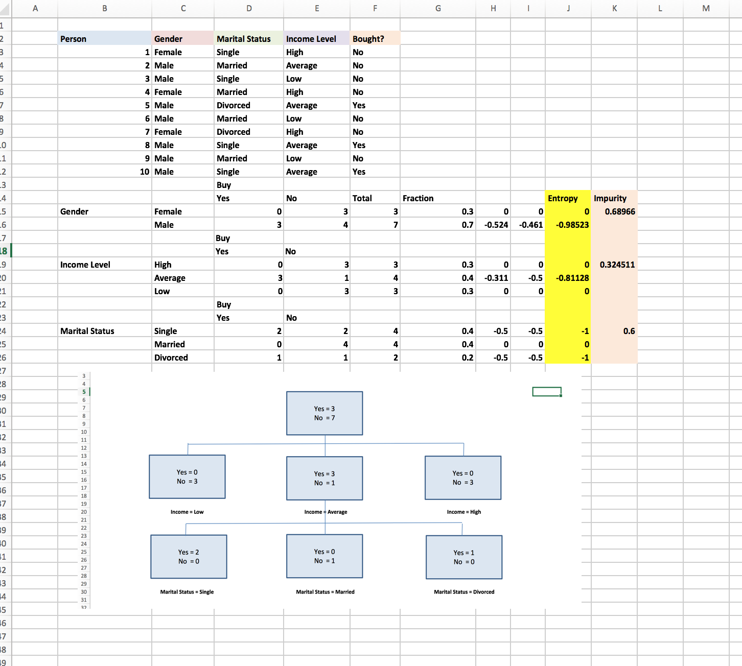
Use the formula =COUNTIFS($C$3:$C$12,$C16,$F$3:$F$12,D$14) to D15:E16 to compute the number of females and males who buy and do not buy Korean spicy ramen.

Then use the formula =COUNTIFS($E$3:$E$12,$C20,$F$3:$F$12,D$14) to D19:E21 to count the number of people for each income level that buy and do not buy Korean spicy ramen.

Use the formula =COUNTIFS($D$3:$D$12,$C24,$F$3:$F$12,D$14) to D24:E26 to count how many people for each marital status buy or do not buy Korean spicy ramen.

Use the formula =SUM(D15:E15) to F15:F26 to compute the number of people for the given attribute value. Use the formula =F15/SUM($F$15:$F$16) to calculate the fraction of observations having each possible attribute value.

To compute for each attribute value category level combination, we will need the equation: P(i|X=a)*Log2(P(i|X=a) combined with IFERROR to ensure that when P(i|X=a)=0 Log2(0) the undefined value will be replaced by zero. In here, we use the formula =IFERROR((D15/$F15)*LOG(D15/$F15,2),0).

Next, to compute the entropy for each possible node split, we use the formula =SUM(H15:I15). To compute the impurity of each split, we use the formula =-SUMPRODUCT(G15:G16,J15:J16).

Step 2: Create Classification Tree
As we can see in this case, the impurity for income level is 0.325 smaller than the impurities of gender (0.69), and marital status (0.6), so we begin the tree by splitting the parent node on income. The Income= Low and Income= High nodes are pure, so no further splitting is necessary. We’ll soon discovered that the Income =Average is not pure, so we need to split this node on either gender or marital status.
Referring back to the calculations we did in Step 1, splitting on gender yields an impurity of 0.811 whereas splitting on marital status yields and impurity of 0. Therefore we splite the Income =Average node on marital status. After that, check when all the terminal nodes are pure, that’s when we’re done. We can create the illustration of this tree using any other software, but for convenience I’ll just use excel.

Step 3: Interpreting the Decision Tree
The tree indicates that if a consumer’s income is low or high, they will not buy Korean spicy Ramen. If the consumer’s income is average and the consumer is married, the person will not buy Korean spicy Ramen. Otherwise, the consumer will buy the product. I guess it somehow makes sense, if you’re married your wife probably won’t let you enjoy junk food like instant noodles. If you have high income, you’d probably eat less fast food and junk food. If you have low income, Samyang Korean spicy ramen isn’t a particularly cheap cup noodle brand.
Jokes aside, this data set is completely made up and random, it’s just fun to try interpreting the numerical results. So there we have our classification tree for segmentation!

